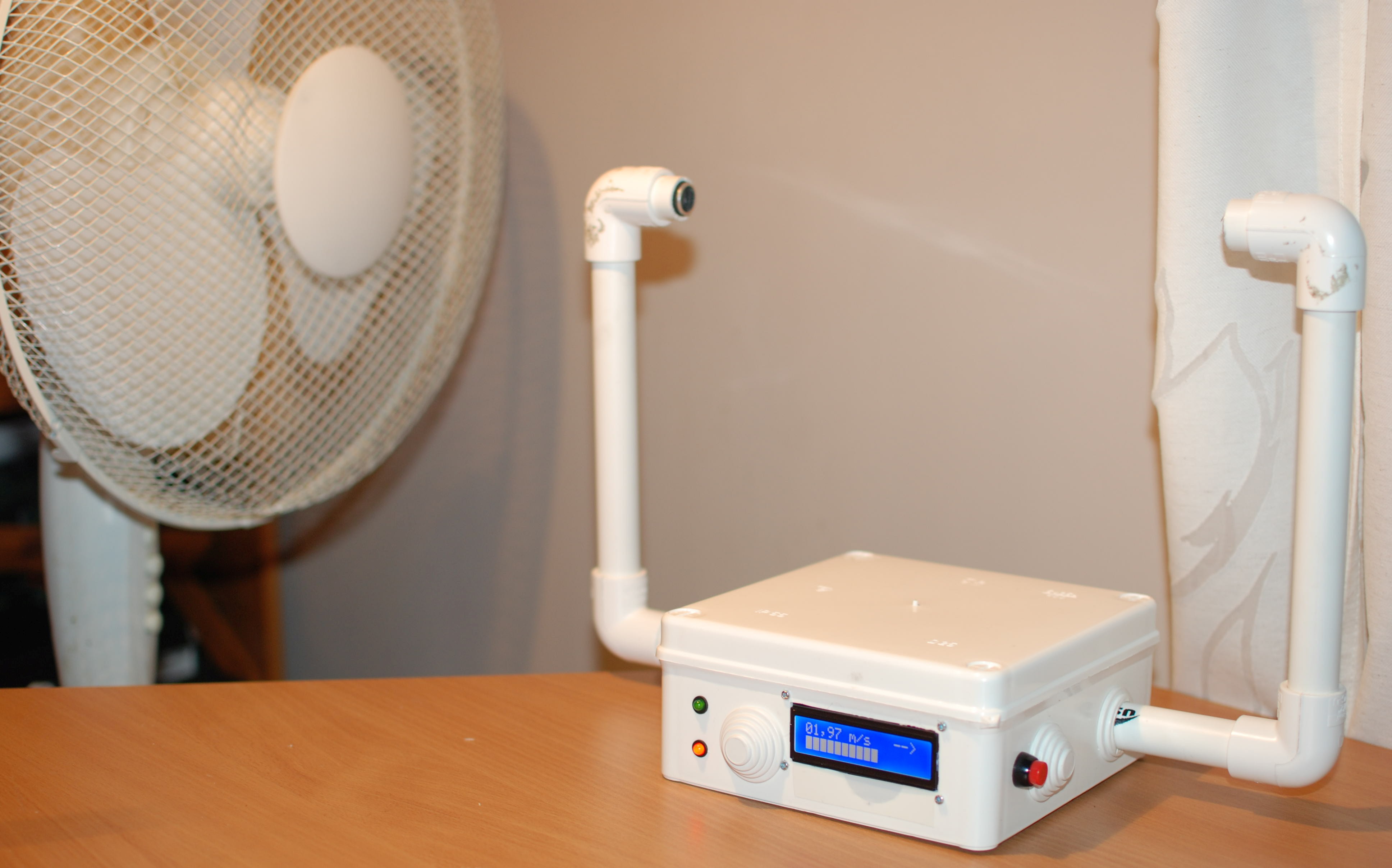
This is Ultrasonic Anemometer project based on AVR ATmega microcontroller.
Principle of operation
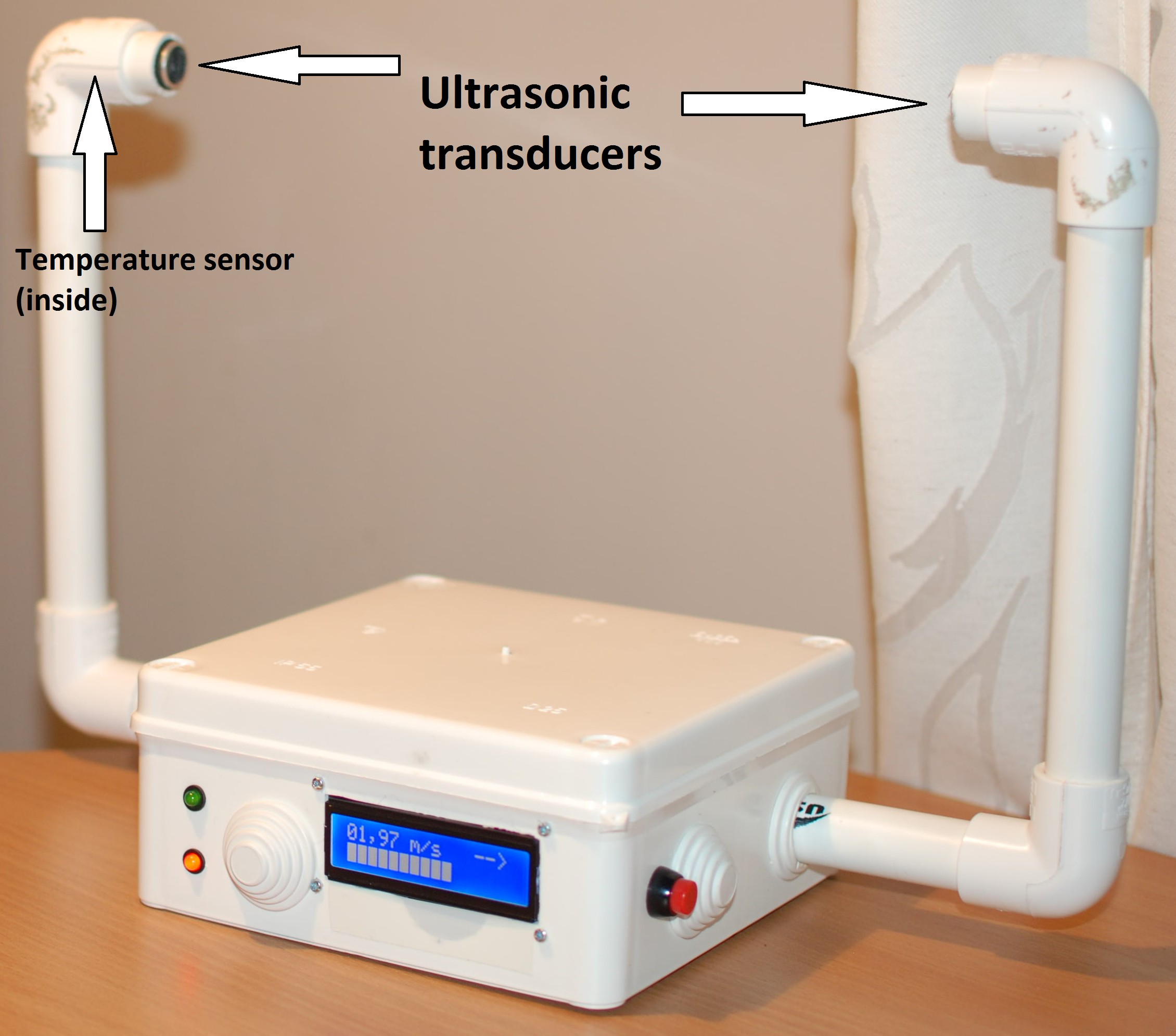
Device measures wind velocity using ultrasounds. Two ultrasonic transducers installed on the end of both pipes send 40 kHz ultrasound signal between each other. Normally the velocity of this signal is the same for both directions. It is equal to the speed of sound, which depends mainly on the air temperature. For dry air and 1000 hPa pressure it can be calculated from:
where:
- vₚ - speed of sound [m/s]
- θ - air temperature [°C]
At 20 °C it is 343,96 m/s.
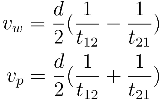
If there is a wind, it alters velocity of sound wave propagating in direction parallel to the wind:

where:
- v₁₂ - velocity of sound wave between point 1 and point 2
- v₂₁ - velocity of sound wave between point 2 and point 1
- vₚ - speed of sound
- vᵥᵥ - speed of wind
Above equations can be transformed into:

The velocity of sound wave can be acquired by measuring time of flight of this wave between ultrasonic transducers. This is what this device does. First transducer emits ultrasonic impulse and second one receives it. Time between those events is measured and later the situation is reversed. Second transducers emits and first one receives.
Knowing distance between those transducers, velocity of sound can be finally calculated.
where:
- d - distance between transducers
- t - time of flight
Velocities in previous equations can be substituted by above time formula:
Anemometer has only two ultrasonic transducers. Therefore, it can only measure wind speed in one direction (parallel to line containing both transducers). Measurement in more dimensions can be achievied by adding more transducers.
Device displays calculated wind speed and its direction on HD44780 LCD display. Under speed value there is a progress bar to next measured value. Unfortunately it takes quite a lot of time to perform all the signal processing calculations on this ATmega (about 46 seconds).
Red LED is lit while power is supplied to the device. Green LED is blinking while the device is working correctly.
Red button on the right performs calibration procedure. After pressing button for 2 seconds, envelope will be calculated of the next set of samples acquired by transducers. The result will be stored in EEPROM and used later for signal processing. This has to be done while there is no wind. Along with samples, temperature from DS1820 sensor is also acquired and stored. This calibration data will survive shutdown of the device because of storage in EEPROM.
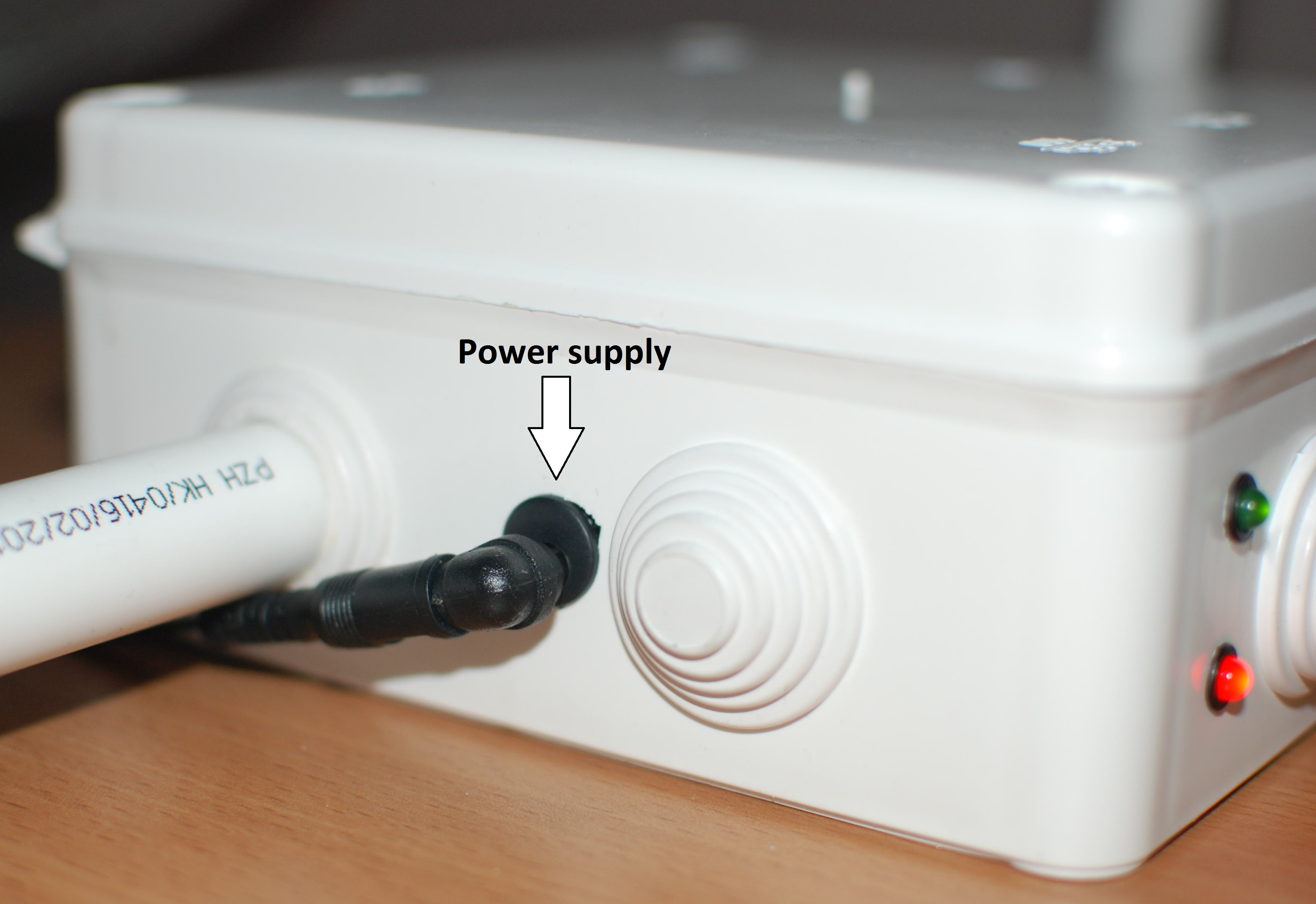
On the left side of the device there is a socket for power supply.

Hardware


Main part of the device is the AVR ATmega1284 microcontroller. It is slightly overclocked for a better performance. I used 24 MHz quartz crystal (official max. frequency is 20 MHz). Controller is programmed with ISP interface. I used simple and cheap USBasp programmer for it.
Calibration button was connected together with resistor, capacitor and diode which do hardware debouncing.
All of the electronics are powered by 5 V supplied by onboard 7805 voltage regulator. It takes voltage straight from power socket. I used external 9 V power supply, but slightly higher voltage would be OK too (not too much to not overheat 7805 regulator). Along with it there is simple protection overcurrent and inverted voltage. Also there is ICL7660 -5 V voltage generator. It’s used for powering multiplexer and operational amplifiers.
HD44780 display is connected in 4-bit mode and busy bit reading.
DS1820 temperature sensor uses 1-Wire interface, but has option for powering it via additional VDD pin. I used this option for better stability.
Analog part of the device needs more explanation. Some of the signals here were measured by an oscilloscope. Microcontroller sends square wave through GENERATOR_OUT line to ultrasonic transducers.
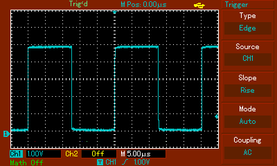
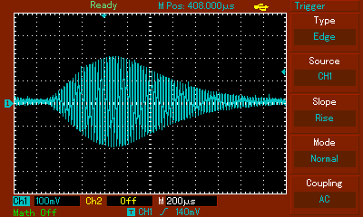
Multiplexer 74HC4052 directs it to either left or right transducer. Multiplexer is controlled by SWITCH_CHANNEL from ATmega. Transducers used in project are narrowband and designed for 40 kHz signal. Experimentally I found out that 40268 Hz signal gives the best amplitude. Transducers are connected with board by shielded cable. While signal from microcontroller is directed to one of them, signal from the other one is directed by multiplexer to amplifiers. Here is the signal before them:

First is an inverting amplifier:

Amplified signal:
Later signal goes to summing amplifier, which again amplifies and adds offset to it. Entire signal has to be voltage positive because ADC used in the device cannot work with negative voltage.

Amplified signal:

For final step I used integrator, which acts as low-pass filter. Any frequencies which are higher than our ultrasonic signal should be filtered out. Transfer function of the filter:
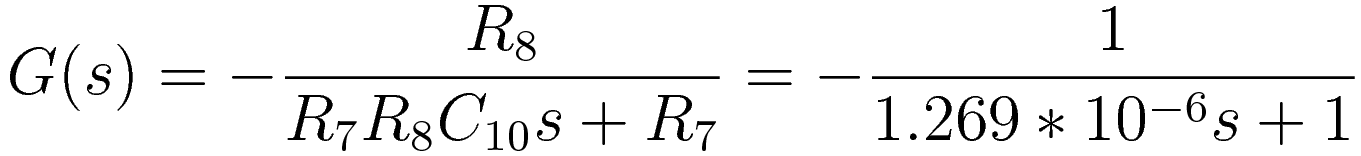
And its Bode plot:

Signal after filtering

After all the operational amplifiers, signal finally goes to ADS7822P analog-to-digital converter. It sends converted digital signal to microcontroller through SPI interface. ATmega here is a master. This ADC has a resolution of 12 bits and max. frequency of 200 kHz. Because of clock dividers in ATmega and clock cycles needed to handle SPI, I managed to get sampling frequency of 157.9 kHz. Nyquist–Shannon–Kotelnikov sampling theorem states that the sampling frequency should be at least 80536 Hz, so it is fulfilled. Analog signal has maximum value of about 4 V, so to increase voltage resolution I attached voltage divider to VREF pin of ADC, which gives voltage of about 4.359 V. This results in voltage resolution of 1.064 mV.
Analog part of the device uses different ground than the rest of the device. It reduces noise derived from high frequency digital signals. Digital ground and analog ground are connected together at one point, close to the power supply.
Electrical schematic and PCB layout were designed using EAGLE application. Tracks on PCB were designed using EAGLE Autorouter. That’s why it’s so ugly :)
Photos of interior:


Signal processing
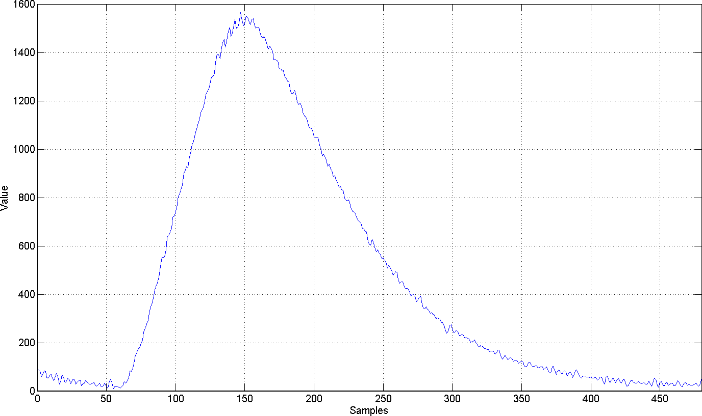
After acquiring by microcontroller, digital samples look like this:
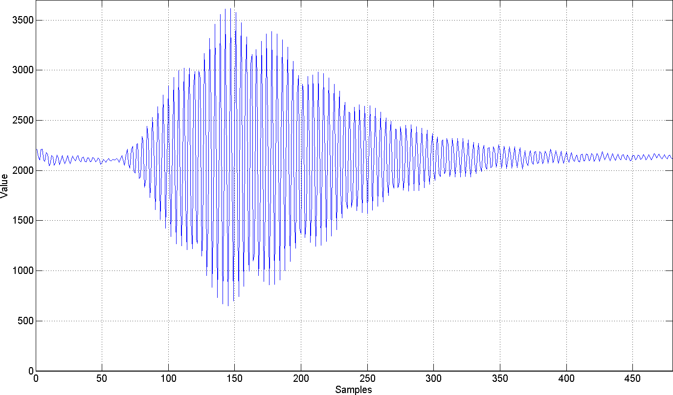
Those samples should be analyzed without offset, so average value is calculated and subtracted from them:

For getting precise time of flight of ultrasonic impulse I decided to calculate envelope of the acquired signal and cross correlate it with the calibration signal stored in EEPROM. To get envelope of signal, a magnitude of its analytic representation can be calculated. To get analytic signal, Hilbert transform has to be calculated first. I used the following discrete formula to acquire it:

where:

and
- x - original signal
- N - number of samples
Analytic signal can now be calculated with the following formula:
Result:
Now the envelope can be cross correlated with the envelope of calibration signal. I used following formula for discrete cross correlation:

Distance between the maximal value and Y axis should determine time of flight of ultrasonic signal:

I also tried calculating only the cross correlation of present and calibration signals, but results were far from being correct. I also tried calculating cross correlation first and then the envelope of it. Results were almost as good as the currently used method, but still they were worse.
I observed that the top part of the calculated cross correlation looks similar to quadratic function. To increase resolution and extract more information from it I decided to use quadratic regression. 31 highest samples are used to approximate quadratic function using following formulas:
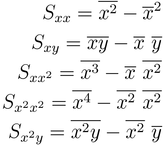
where:
- x - function arguments
- y - function value
- ( ¯ ) - average value
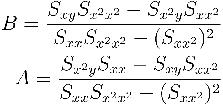
Coefficients can now be calculated (coefficient C is not needed):
And finally maximum of the function can be calculated:
This maximum is used to calculate the time of flight. Here is comparison of signal and approximated quadratic function:

Distance between the maximal value and Y axis multiplied by 6333 ns results only in signal time of flight difference between conditions with wind and without wind. To get total time of fligh there has to be added time of flight during windless conditions. This time is calculated using temperature acquired during calibration by using formula from the beggining of the article. Distance between transducers also has to be known. It’s 27 cm. Any later temperature changes should not affect the final result.
Knowing the total signal time of flight, final wind speed value is calculated.
Software
Software for the ATmega1284 microcontroller was developed using Atmel Studio IDE with AVR8 GNU Toolchain. It contains avr-libc libraries and avr-gcc compiler. Optimization flag -Os was set for compilation. All used flags are below:
avr-gcc -x c -funsigned-char -funsigned-bitfields -DNDEBUG -DF_CPU=24000000UL -Os -ffunction-sections -fdata-sections -fpack-struct -fshort-enums -mrelax -Wall -mmcu=atmega1284 -c -std=gnu99 -MD -MP -MF "$(@:%.o=%.d)" -MT"$(@:%.o=%.d)" -MT"$(@:%.o=%.o)"
Fuse bits are configured as follows:
| Fuse Low | Fuse High | Extended Fuse |
|---|---|---|
| 0xF7 | 0xD1 | 0xFC |
Pretty online fuse calculator showing this configuration is here. Fuse Low is configured to allow clock source from 24 MHz quartz crystal. Fuse High, among other things, disables JTAG interface, so more pins can be used as GPIO. Extended Fuse enables Brown-out detection at level 4.3 V.
One of the most important fragment of code is shown below:
inline void getDataFromAdc(uint16_t *data) {
  // Activating ADC.
  SPI_SS_LOW;
  // Starting transmission.
  SPDR = 0x00;

  // Waiting for end of transmission.
  // NOP causes loop to check end of transmission flag at the most optimal time.
  asm volatile("nop"::);
  while(!(SPSR & _BV(SPIF)));

  // Starting another transmission.
  SPDR = 0x00;
  // Saving byte from previous transmission.
  *((uint8_t*)data + 1) = SPDR;

  // Waiting for end of transmission. This time three NOP's were needed.
  asm volatile(
    "nop\n\t"
    "nop\n\t"
    "nop\n\t"::
  );
  while(!(SPSR & _BV(SPIF)));

  // Saving byte from transmission.
  *((uint8_t*)data + 0) = SPDR;
  // Deactivating ADC.
  SPI_SS_HIGH;
}
This function is responsible for acquiring samples from ADC. Execution time of it is significant, because sampling frequency depends on it. SPI_SS_LOW macro drives SS line low on SPI interface. It enables ADC. Afterwards, writing 0 to SPDR register begins transmission. Microcontroller is transmitting this 0 over MOSI line (which is not even connected to ADC), but at the same time, it receives data byte over MISO line. while(!(SPSR & _BV(SPIF))) waits for the end of transmission. Because checking for SPIF flag in loop takes a few clock cycles, adding asm volatile(“nop”::) ensures that the flag is checked right after end of transmission. This solution was found by analyzing assembly code during simulator debugging. Right after that, another transmission starts. Afterwards, previous byte is saved in variable. SPDR register for transmitted byte is different than SPDR for received byte, so this sequence was used just to save some clock cycles. SPIF is checked again for end of transmission, but now three NOPs were needed. Later, new byte is saved in variable and SPI_SS_HIGH drives SS line high and disables ADC. Restarting ADC is needed between every sample.
Generated assembly from above code is shown below:
cbi    0x05, 4
out    0x2e, r1
nop
in     r0, 0x2d
sbrs   r0, 7
rjmp   .-6
out    0x2e, r1
in     r18, 0x2e
movw   r30, r24
subi   r30, 0xA7
sbci   r31, 0xFE
std    Z+1, r18
nop
nop
nop
in     r0, 0x2d
sbrs   r0, 7
rjmp   .-6
in     r18, 0x2e
st     Z, r18
sbi    0x05, 4
adiw   r24, 0x02
cpi    r24, 0xC0
ldi    r18, 0x03
cpc    r25, r18
brne   .-52
Execution of this code takes exactly 152 clock cycles. For 24 MHz clock, it gives 6333 ns. It is equivalent to sampling frequency of 157.9 MHz.
In this program there are no floating point numbers, because ATmega microcontrollers don’t have hardware support for them, which would result in very long computation time and large memory consumption. Trigonometric functions needed for calculations were implemented as lookup tables.
Conclusion
I tested the device with typical household fan. Result of the measurements seem to be OK. Unfortunately I don’t have access to any professional hardware, which would verify it.
46 seconds needed for calculating wind speed is a bit too long time. More powerful microcontroller should have been used or a different signal processing method. ATmega microcontrollers are very slow comparing to modern ones.
Despite it, while creating this device I learned many new things about electronics, digital signal processing and programming embedded systems in C. Also I Learned how does ultrasonic anemometer works.

Ultrasonic Anemometer by Karol Leszczyński is licensed under a Creative Commons Attribution-ShareAlike 4.0 International License.